stat_error() and sign_aware + demo

library(ggplot2)
library(ggerror)

set_theme(
  theme_minimal() + theme(
  plot.title = element_text(hjust = 0, family = "consolas", size = 12),
  axis.title = element_blank()
))

Version 1.0.0 adds two new features:

• stat_error() computes error bounds directly from raw data. It follows ggplot2’s fun.data contract, meaning it works with any summary function you pass in - mean_se, mean_ci, or a custom one (see details below).
• sign_aware = TRUE interprets the sign of input values as direction. Positive and negative values are mapped to error_pos and error_neg, respectively. This is useful when plotting residuals or any signed quantity where direction carries meaning.

stat_error():

Pass raw observations and let the stat compute the error. The default is mean_se - mean with one standard error:

ggplot(mtcars, aes(factor(cyl), mpg)) +
  stat_error()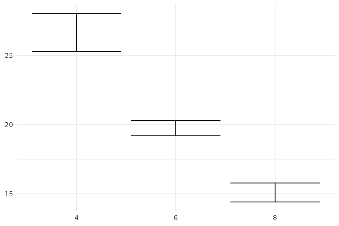

mean_ci for a 95% confidence interval:

ggplot(mtcars, aes(factor(cyl), mpg)) +
  stat_error(fun = "mean_ci", error_geom = "pointrange")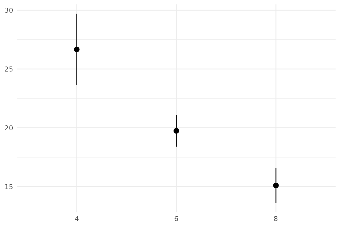

Both mean_ci and mean_se accept na.rm as an argument. mean_ci also accepts conf.int, default is 0.95.

Custom summary function

You can also pass a custom function following ggplot2’s fun.data syntax — it takes a numeric vector and returns a single-row data frame with columns y, ymin, ymax:

iqr <- function(y, type = 6) {
  data.frame(
    y    = median(y),
    ymin = stats::quantile(y, 0.25, names = FALSE, type = type),
    ymax = stats::quantile(y, 0.75, names = FALSE, type = type)
  )
}

ggplot(mtcars, aes(factor(cyl), mpg)) +
  stat_error(fun = iqr, type = 1)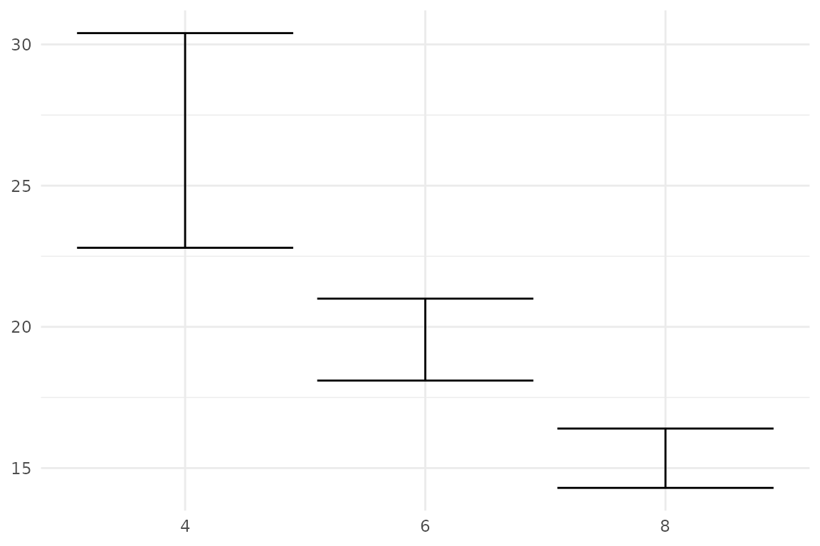

You can pass an arbitrary number of arguments to stat_error().

While geom_error uses stat = 'identity', you could also pass stat = 'error', which is equivalent to stat_error().

sign_aware: residuals as one-sided bars

I really love this usecase. Drawing sign-aware errors (with colours!) used to be a pain. Not anymore!

• First, let us fit a (dummy) model

model <- lm(mpg ~ wt, data = mtcars)
mt_model <- mtcars
mt_model$predicted <- fitted(model) # predicted values (y_hat)
mt_model$res <- resid(model) # raw distances (y-y_hat), some positive, some negative

ggplot(mt_model, aes(mpg,predicted)) +
  geom_point() +
  geom_abline(slope = 1, intercept = 0) +
  geom_error(aes(error = res), sign_aware = TRUE, orientation = "x",
             colour_pos = "firebrick", colour_neg = "steelblue")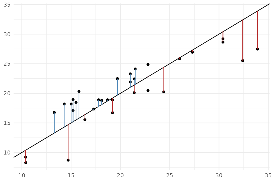

*Since both axes are numeric, ggerror can’t infer the orientation itself, so we have to pass it